The “Inscriptions of Israel/Palestine” (IIP) dataset is an online database which seeks to make all of the previously published inscriptions of Israel/Palestine from the Persian period through the Islamic conquest (ca. 500 BCE - 640 CE) freely accessible [Satlow 2022]. This database includes approximately 4,500 inscriptions, and they are written primarily in Hebrew, Aramaic, Greek and Latin, by Jews, Christians, Greeks, and Romans. Some of the examples include imperial declarations on monumental architecture, notices of donations in synagogues and humble names scratched on ossuaries [Satlow 2022]. Each inscription exists as a single XML file structured according to EpiDoc conventions [Elliott, Bodard, Cayless, et al. 2006].

We consider the following characteristics in the dataset:

It is worth noting that language, material, and region are objectively determined in most cases. Dating, on the other hand, is often determined subjectively by scholars; relatively few contain dates or were found in carefully controlled archaeological excavations. Thus, we examine how machine learning models can accurately predict the date of inscriptions given the information of other variables in the dataset. All variables inside the dataset except date are categorical, as they are not quantifiable.

The IIP dataset is converted into a single csv file through using the ElementTree XML API in Python programming. One of the features of the IIP dataset, like many others in the humanities, is that it contains a number of categorical variables, that is, different phrases that occur within a single XML element. For example, there are many different cities in the location element, and over fifty different text genres (e.g., funerary, dedicatory, label, prayer) are found within the appropriate element. The result of this is an imbalanced dataset. Imbalanced datasets occur when the proportion of minority class is significantly low compared with other classes in the dataset, and creating an effective machine learning algorithm with imbalanced datasets is a very difficult problem [Johnson and Khoshgoftaar 2019]. It is also important to make sure that all the possible categorical values are in the training dataset to create a good machine learning model. For example, if the training set does not include any inscriptions that has the city name “Jerusalem”, it would be difficult for the machine learning algorithm to use the Jerusalem information in the test dataset. Error messages can come out in many machine learning programs when they encounter some information that is not included in the training dataset. Splitting the dataset into training and test set is done randomly, so it is possible for the minority class to not appear in both training and test set if the number of observations from the minority class is small. To have enough observations in the minority class, we combine various unique terms and generate a dataset that is better suited for the machine learning algorithm.

We first fix spelling mistakes inside the dataset. Afterwards, we combine words that describe the same concept. For instance, “Golan Heights” and “Golan” can be grouped together as “Golan” and there is no need for the machine learning algorithm to consider these elements separately. There are also some phrases such as “dedicatory quotation” and “dedicatory verse”, where they describe different objects but can be grouped together as “dedicatory” to reduce the number of variables inside the dataset. However, we take a different approach with the “City Name” variable. There are 244 unique city names inside the dataset, and many of them only include a few inscriptions. Since the location of inscription is already indicated in the “Region” variable, we only consider “Jerusalem” and “Other Cities” to make the prediction easier to interpret. We also do not consider all variables in the dataset, such as condition of artifacts and relief style, as they have a lot of missing values.

We use a technique called one-hot encoding to convert the categorical features to numerical features. There are many machine learning algorithms that can only analyze numerical data, so analyzing categorical variables without one-hot encoding can cause some issues. In this technique, we create a binary column for each category, where we denote the output of the column to be 1 if the variable is present and 0 if the variable is not present. For example, we create a new variable called Language_Greek to describe if the inscription is written in Greek or not. The Language_Greek variable will be 1 if the inscription is written in Greek, but 0 otherwise.

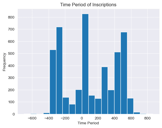
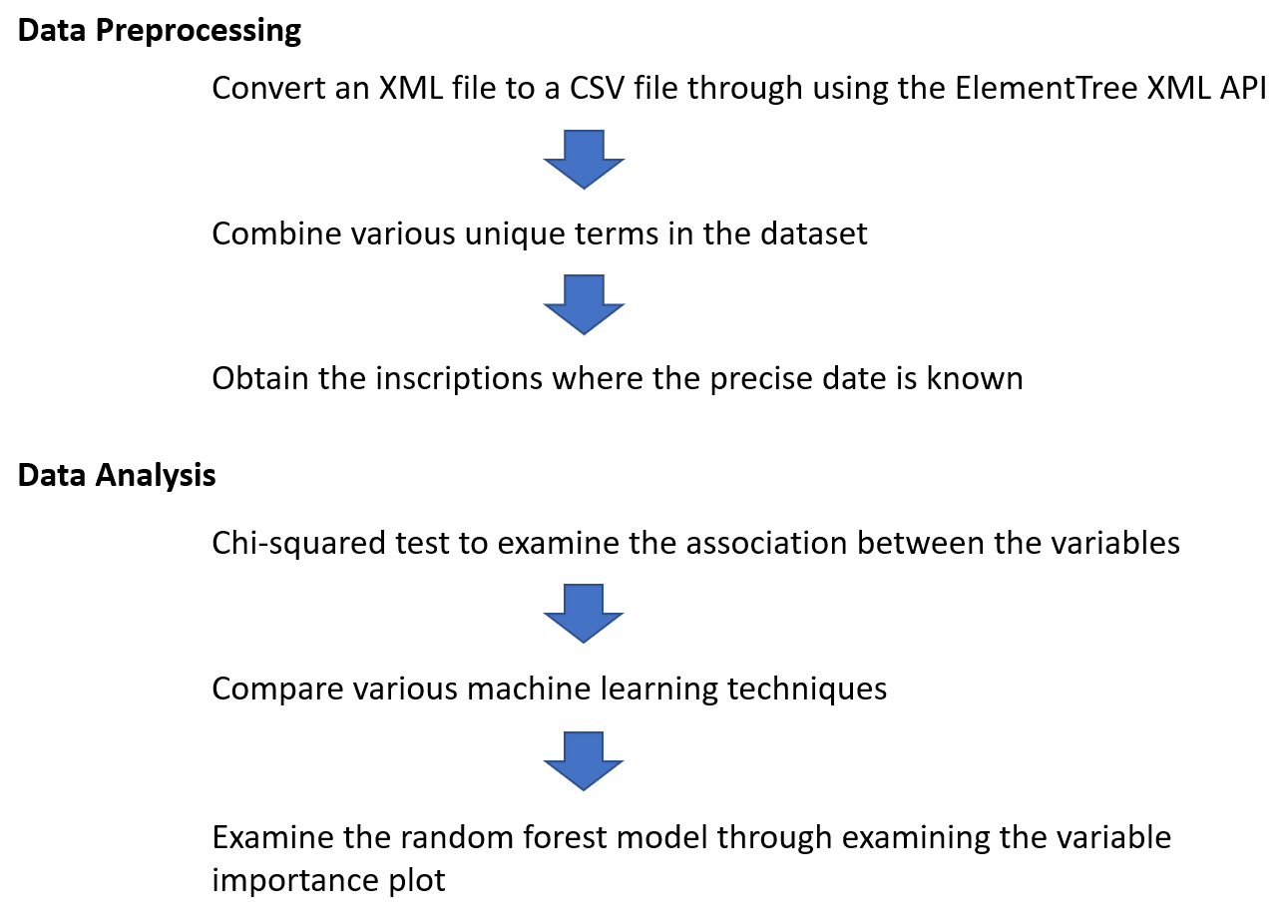
These inscriptions are used to examine the performance of machine learning models to predict the time periods. The time period distribution of inscription is shown in Figure 1. The mean date is 109.68 CE with standard deviation 311.47. The large standard deviation implies that the dataset is suitable for conducting this analysis, as it has inscriptions from a wide range of time periods. After we preprocess the dataset, we select 650 inscriptions that actually contain a certain date. The overview of the steps that are taken in this research project is shown in Figure 2.

We compare the performances of eleven machine learning models: linear regression, ridge regression, lasso regression, elastic net, decision tree, random forest, neural network, XGBoost, and support vector regression with linear, radial and polynomial kernel. We select these algorithms, as they require minimal hyperparameter tuning and do not require data transformation. Hyperparameters determine the overall behavior of the machine learning model, and they must be set appropriately by the user before conducting the analysis [Claesen and DeMoor 2015]. Hyperparameter tuning is often performed manually, but it is impractical when we have many hyperparameters, and technical expertise is required to correctly set the hyperparameters [Claesen et al. 2014]. To create a simple and reproducible machine learning prediction model, we try to select models that do not require fine parameter tuning.

We will provide a brief overview of these techniques with some examples of previous studies in digital humanities. Readers who are interested in further details of machine learning techniques should consult Hastie et al. [Hastie et al. 2009].

Metrics are used to quantify the accuracy of the machine learning model once we obtain the machine learning models. We will examine three commonly used metrics to evaluate the machine learning algorithm, root mean square error (RMSE), mean absolute error (MAE), and R-squared. 10-fold cross-validation is performed to compare the performances of machine learning algorithms. In k-fold cross validation, we split the dataset into k smaller sets with equal number of elements and use k-1 sets to train the model, while the remaining set is used to evaluate the model [Hastie et al. 2009]. We repeat the above iteration thirty times and compute the mean value of the determined metrics in cross validation to determine the optimal machine learning model for predicting the date.

We use R version 4.1.3 to perform the data analysis and Python version 3.8.3 to obtain the XML dataset from the IIP database [Satlow 2022]. The dataset and the codes that we use to obtain the dataset are openly available to the public at https://github.com/daikitag/Inscriptions-of-Israel-Palestine.

It is important to understand the relationship between the predictor variables in the dataset before conducting machine learning analysis, as we can understand the issues behind effectively analyzing the dataset. Considering that all predictor variables are categorical, we use Pearson's chi-squared test of independence to examine the association between the variables in the dataset. We have examined the association between:

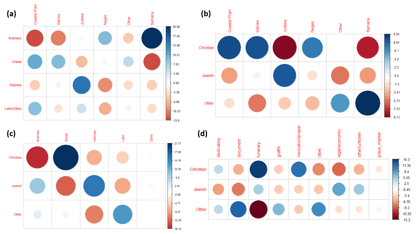
The residual plots of the chi-squared test are shown in Figure 3. Results from chi-squared test indicate that there is a significant relationship between all the examined combinations (p<0.001).

The results imply that the predictor variables are correlated with each other, which raises the problem of multicollinearity. Multicollinearity occurs when independent variables in the regression model are correlated with each other [Alin 2010]. One of the key assumptions of the linear regression model is that the predictor variables are uncorrelated. Thus, multicollinearity can undermine the statistical significance of an independent variable and can give inaccurate coefficient estimates when traditional statistical techniques are used [Allen 1997].

In contrast, due to recent advances in machine learning techniques, it has been reported that machine learning can better analyze data with multicollinearity than traditional statistical techniques [Chan et al. 2022]. The presence of multicollinearity suggests the usage of machine learning techniques to effectively analyze the dataset.

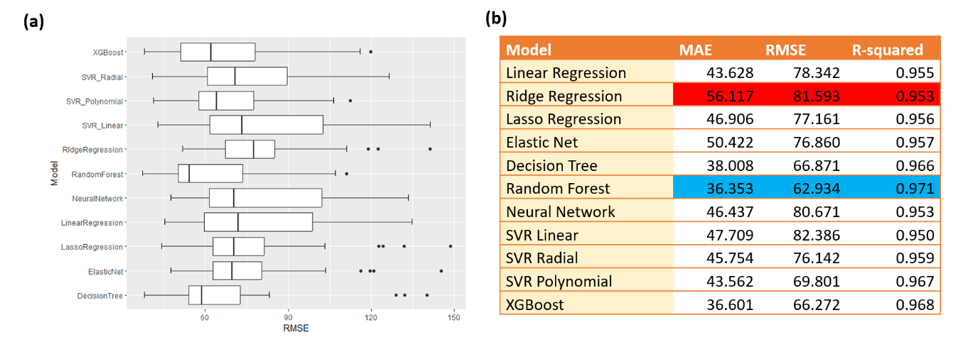
A total of eleven regression models are compared: linear regression, ridge regression, lasso regression, elastic net, decision tree, random forest, neural network, SVR linear, SVR radial, SVR polynomial, and XGBoost. The optimal hyperparameters of the machine learning algorithms are determined through 10-fold cross-validation. The cross-validation procedure is repeated 3 times, and the machine learning model is tested by using a total of 30 different datasets, each of which are generated through cross-validation. The evaluation results are shown in Figure 4, where Figure 4 (a) shows the distribution of RMSE from 30 different datasets and Figure 4 (b) shows the mean values of MAE, RMSE and R-squared. MAE and RMSE measure the error of the machine learning model and R-squared is a goodness of fit measure. The random forest model has the lowest value for MAE and RMSE, and has the highest value for R-squared among all models that are examined. This implies that random forest model is the optimal model for predicting the date of inscriptions.

We describe the random forest model in detail, as it is the best model that is implemented in the previous section. We initially convert the number of trees that the random forest model generates from 100 to 1000 to determine the optimal number of trees that we put inside the algorithm, but we do not observe any significant differences. Thus, we select 500 number of trees, as it is the default number of trees in R's randomForest package [Liaw and Wiener 2002].

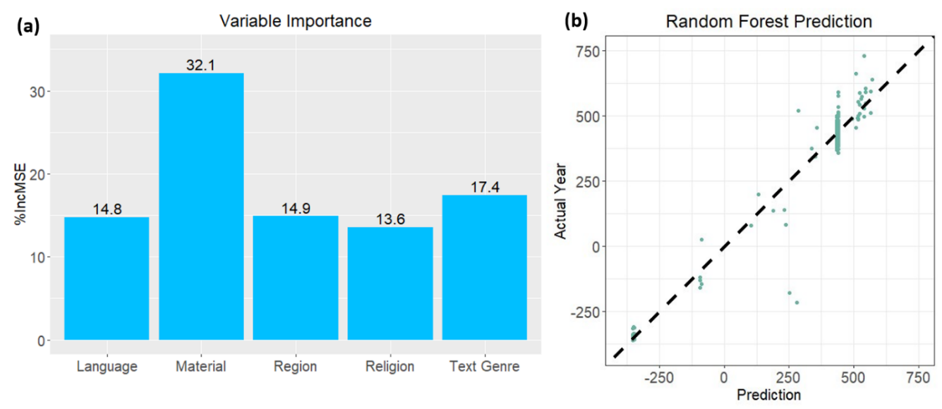
Figure 5 (a) shows the variable importance plot of the random forest model. Variable importance is based upon the mean increase of mean squared error as a result of permuting a given variable [Liaw and Wiener 2002]. The plot suggests that the material of inscription is the most important variable in the prediction model. The prediction plot is shown in Figure 5 (b). The machine learning model is trained based on the training dataset, which includes 70% of the randomly chosen inscriptions in the data. The prediction plot is created by using the test dataset, which is not used to train the machine learning model.

Every region and community in the Mediterranean in antiquity had its own epigraphic characteristics. The statistical analysis reveals some features of different communities within Judea/Roman Palestine. From the residual plot in Figure 3 (a), we can infer that inscription in Judea have a higher probability of being written in Hebrew and inscriptions in Negev have a higher probability of being written in Aramaic. There is also a very strong positive association between Aramaic and Samaria. However, there is a lower probability of Aramaic inscriptions found in the Coastal Plain.

When we examine the residual plot in Figure 3 (b), there is a higher possibility of discovering Christian inscriptions in Coastal Plain, Galilee, and Negev. There is a higher possibility of discovering Jewish inscriptions in Judea and Galilee. However, the probability of finding Christian and Jewish inscriptions in Samaria is lower than other regions, and there are many inscriptions from other religions. These results are consistent with what we would expect from other historical sources.

The residual plot of language and religion is shown in Figure 3 (c). Christian inscriptions have a strong positive association with Greek, but negative association with other languages, specifically Aramaic. Inscriptions written in Aramaic and Hebrew are more likely to be Jewish inscriptions.

The relationship between text genre and religion is shown in Figure 3 (d). The plot implies that Christian inscriptions tend to be funerary or invocation related compared with other religions, but the probability of Christian inscription being document or legal/economic is lower. It seems that Christian inscriptions tend to be more religious and less administrative.

We are able to conclude that the random forest model is the optimal machine learning model for predicting time periods of inscriptions. This is consistent with previous research, as it has been reported that tree-ensemble algorithms like random forests are better to analyze tabular data [Shwartz-Ziv and Armon 2022], which is the data type that we use in our project. If we examine the metric values in Figure 4 (b), we see that random forest, XGBoost and decision tree perform better than other models that we have examined. This highlights the importance of using tree based machine learning algorithms to analyze tabular dataset.

Our study also shows that linear models do not perform well compared with other methods in analyzing tabular datasets which consists of only categorical variables. This might be due to the nonlinear interactions between the variables in the dataset. In terms of SVM, it is important to select the appropriate kernel for each dataset. In our example, we see that SVR with linear kernel performs the worst out of all three kernels that we have examined. However, there are many kinds of kernels in SVM, and it would be a challenging problem to select the optimal kernel for the dataset. The results also suggest that the predictability of neural network is not high compared with tree-based algorithms when we analyze tabular datasets. Many digital humanities datasets are tabular data and they are rarely large enough to effectively train the deep learning algorithm. Our results are consistent with the previous study by Shwartz-Ziv & Armon [Shwartz-Ziv and Armon 2022], where they also showed that tree ensemble methods are better than deep learning techniques to analyze tabular data.

In contrast, a random forest model can easily be implemented by specifying two hyperparameters of the model, and it is possible for a random forest model to capture the nonlinear interactions inside the dataset. This is a major advantage of random forests, as most machine learning models require fine tuning of hyperparameters [Hastie et al. 2009].

In spite of advances in machine learning techniques, it is still necessary to have epigraphers to analyze inscriptions. According to the variable importance plot of the random forest model (Figure 5 (b)), material is the most important variable in making predictions, but we cannot ignore the effects of other variables, including religion and text genre. These variables are subjective, and necessitates the importance of having humans to classify the inscriptions as well. Even in the research project conducted by Assael et al. [Assael et al. 2022], they showed that accuracy was the best when the deep learning algorithm was paired up with historians. Machine learning algorithms are still not perfect, so it would be important for us to incorporate knowledge from both human scholars and computers to analyze the dataset effectively.